CaTSper Full Documentation
CaTSper Step-by-step Tutorial
This tutorial introduces the CaTSper tool and how to use it to calculate the frequency dependent absorption cofficient and refractive index spectra from a set of sample and reference time-domain waveforms, that were previously converted into the .thz file format using the CambridgeTHzConverter tool. Please also refer to the CaTSper Processing Steps documentation where the mathematical steps Catsper uses are outlined.
- CaTSper Step-by-step Tutorial
To Convert the Project Data
Please follow the instructions in the CambridgeThzConverter tutorial documentation to generate a .thz file before using Catsper.
To Load/Remove a Project into Catsper
Check the .thz file properties
Please ensure the “Name” row in the “Tcell” array has been correctly assigned with certain distinguishable value for each waveform recorded, otherwise, nothing will be displayed in the “Measurement” list box in the Catsper user interface. This can be done by loading the .thz file back into the “Catspet THz Converter”.
Import the .thz file to Catsper
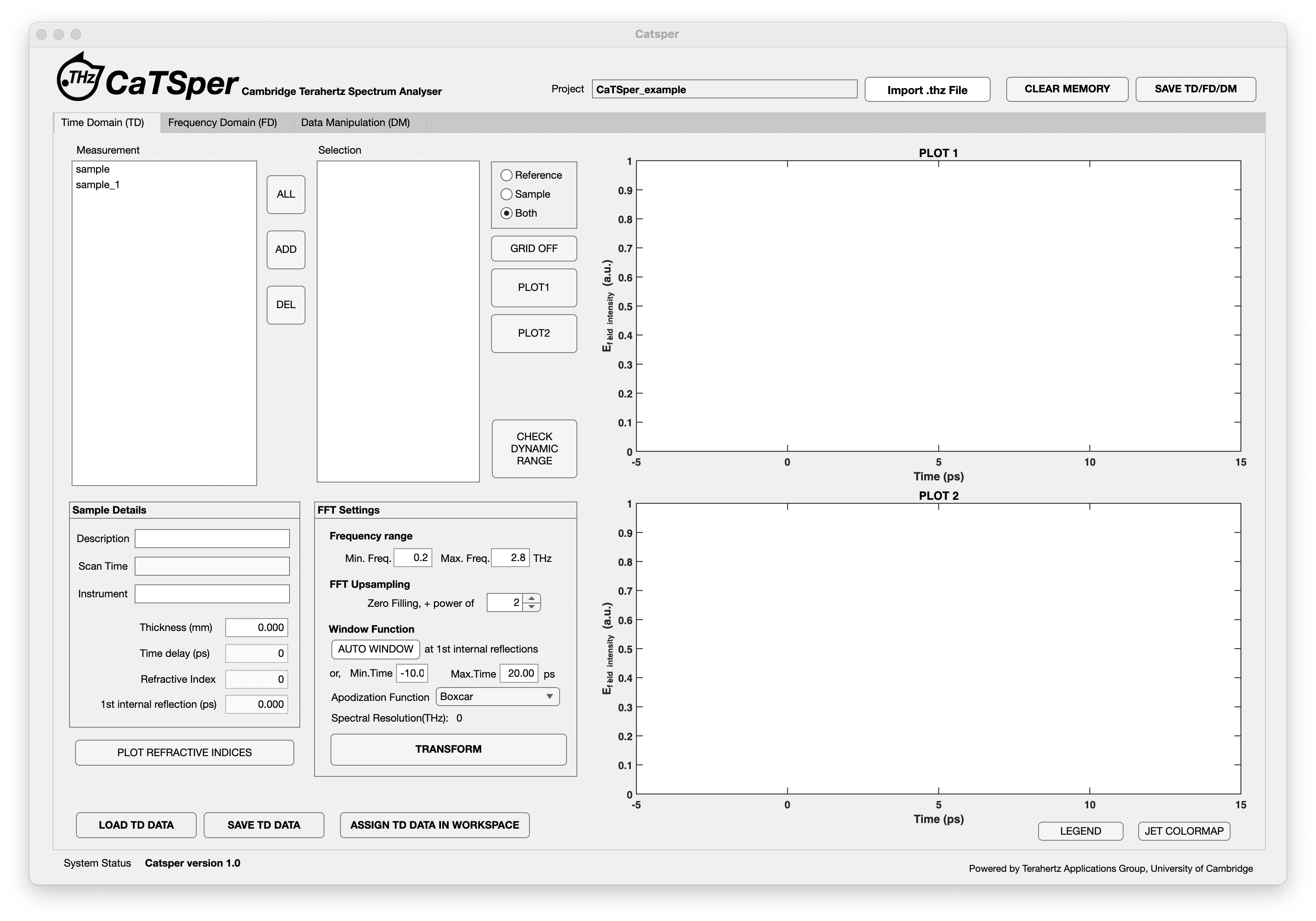
Click the “Import Catsper .thz file (Tcell)” button at the top of the Catsper user interface and selected the .thz file created by the “Catspet THz Converter”. The “Project” edit field will display the name of the file imported without the “.thz” suffix. If the measurements (or terahertz waveforms recorded) are assigned with certain names, they will all appear in the “Measurement” list box. Otherwise, please check the .thz file properties.
The user will see the following UI if the data have been successfully imported into Catsper:
Clear the app memory and remove all existing data
Click the “CLEAR MEMORY” button at the top of the Catsper user interface. A dialogue box will pop out to confirm this action “Do you want to clear memory?”
A “Yes” answer will remove all entries and items from the “Measurement” and “Selection” list boxes and reset the MATLAB workspace. A “No” or “Cancel” answer will keep the existing data and take the user back to the Catsper user interface.
Time Domain (TD) Tab
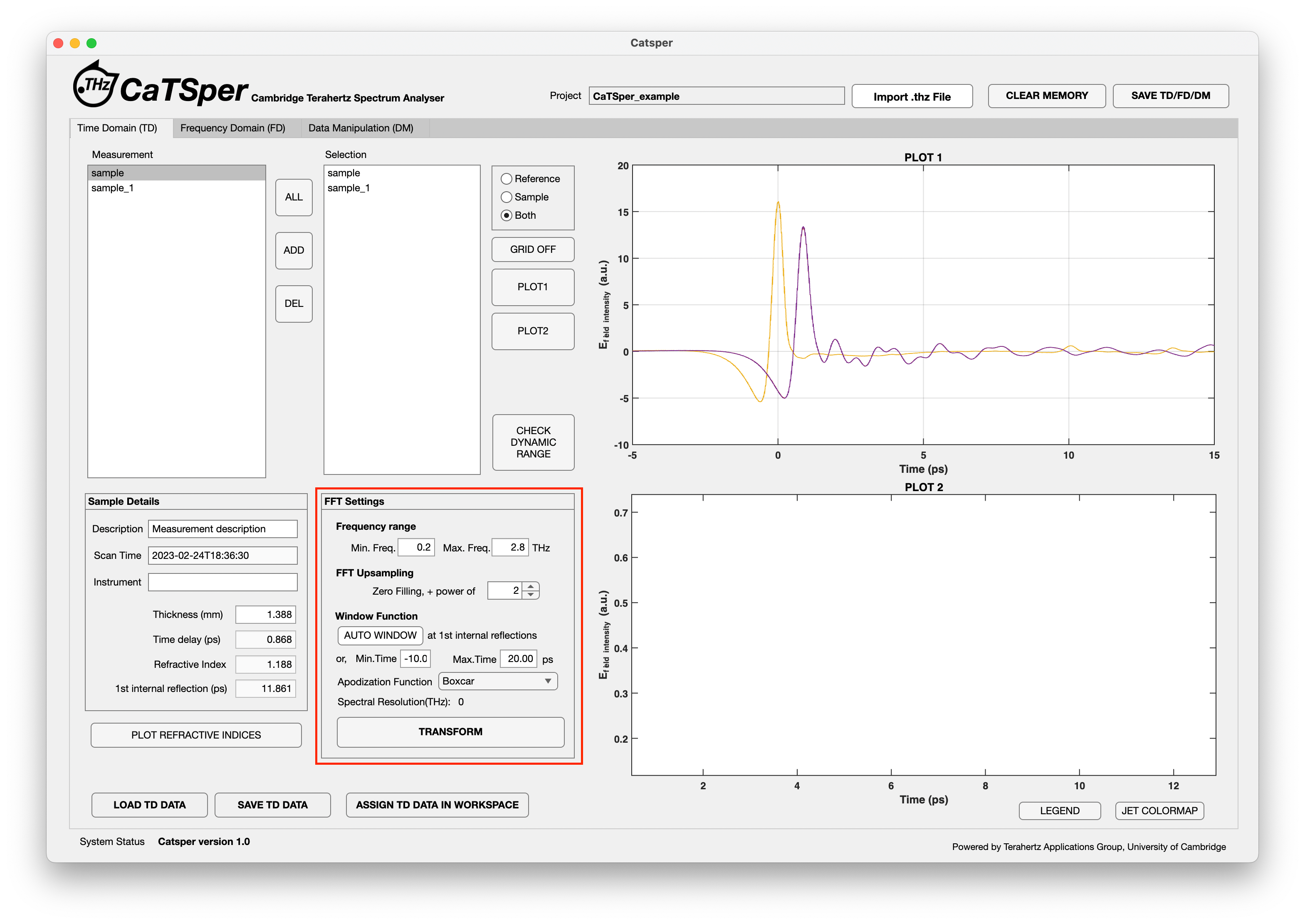
The default tab at the top left corner selected is the “Time Domain (TD)”. If another tab is selected, the user needs to click the “Time Domain (TD)” tab to open the TD analysis page.
Choose the measurement for analysis
Once all measurements are listed, the user can pick those of interest by click the target item (and the selected item will be shaded). In the “Sample Details” field, the following measurement details are shown: “Description”, “Scan Time”, “Thickness (mm)”, “Time Delay (ps)”, “Refractive Index” and “1st internal reflection (ps)”.
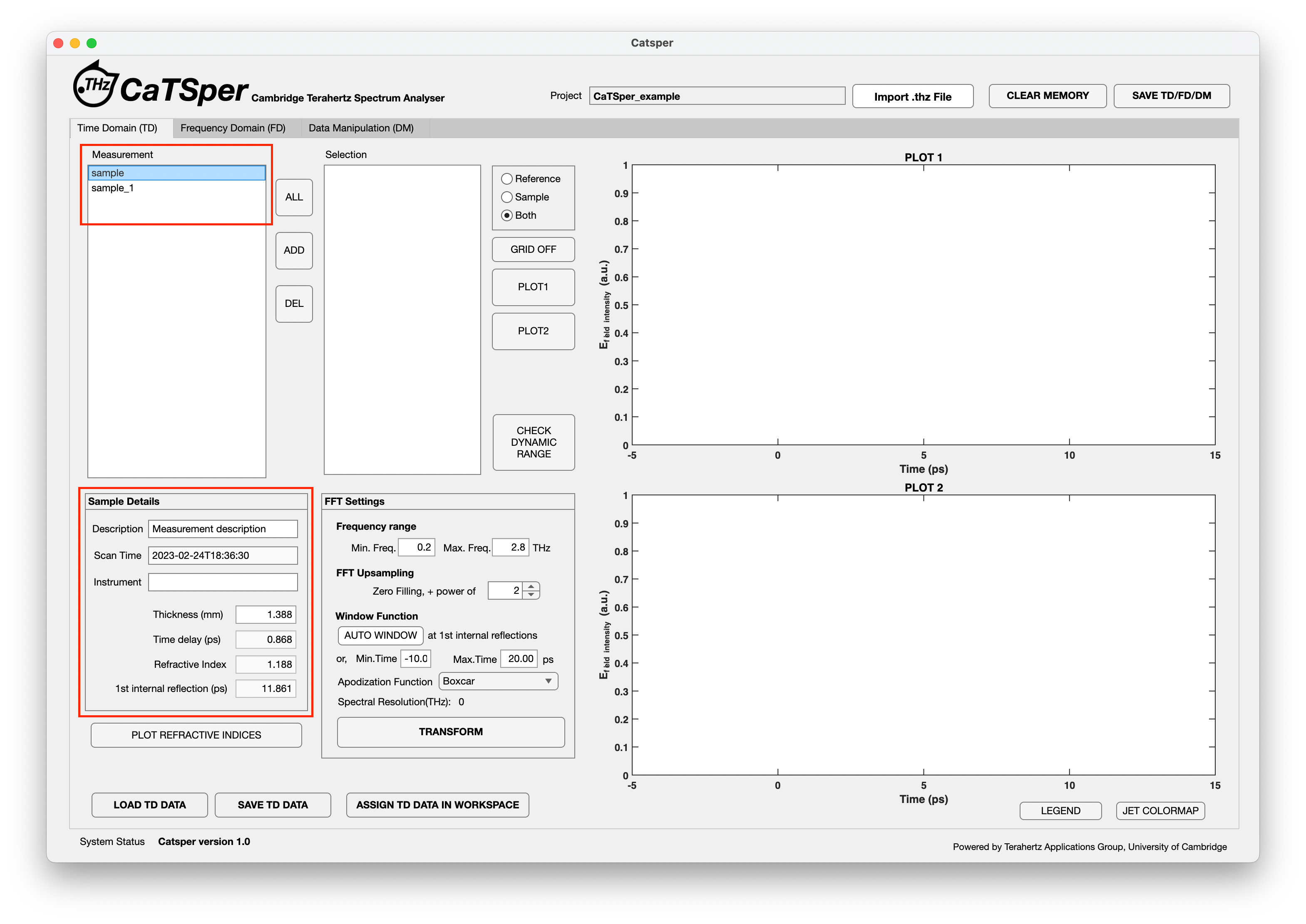
The user can manually change the “Description” and “Thickness (mm)” edit field, and the latter one allows the “Refractive Index” and “1st internal reflection (ps)” to be automatically computed once a new positive value has been assigned to the “Thickness (mm)” edit field.
The calculations in these fields can be found here.
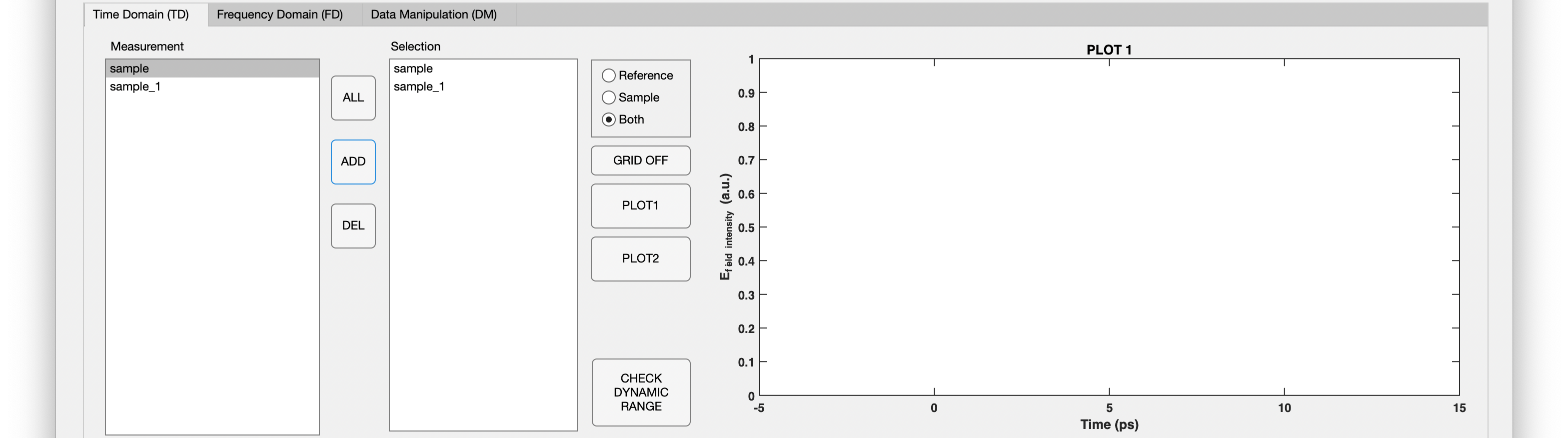
To add this measurement to the “Selection” list box, the user can click the “ADD” button and measurement name will then appear in the “Selection” list box. Please note that only one measurement can be selected each time, so if you want to include all measurements, simply click the “ALL” button and all measurements will be added thereafter. If you want to remove some measurements already in the “Selection” list box, choose the target item in the “Selection” list box and click the “DEL” button. This item will then disappear from the “Selection” list box, however, it can still be found in the “Measurement” list box.
Save the list of measurements
This functionality allows the user to pause the analysis and return at a later stage. Once the time-domain data have been selected and appeared in the “Selection” list box, the user can click the “SAVE TD DATA”. A message box will pop out to ask: “Do you want to save all data?”. If the user return “Yes”, then all list items in the “Measurement” list box will be saved in the .thz file, whereas “No, only the selected data” will only save those in the “Selection” list box.

Load the list of measurements
Click the “LOAD TD DATA” and choose the .mat file created by the “SAVE TD DATA” functionality. The measurements saved in this file will then be imported to the “Measurement” and “Selection” list boxes.
Plot the TD data
The plot can only be done once the data are selected and displayed in the “Selection” list box. Clicking the “PLOT1” button will generate the waveform plot on the “PLOT 1” axis whilst such plot will appear on the “PLOT 2” axis if the “PLOT2” button is pushed in. The user can plot the same measurement on both axes.
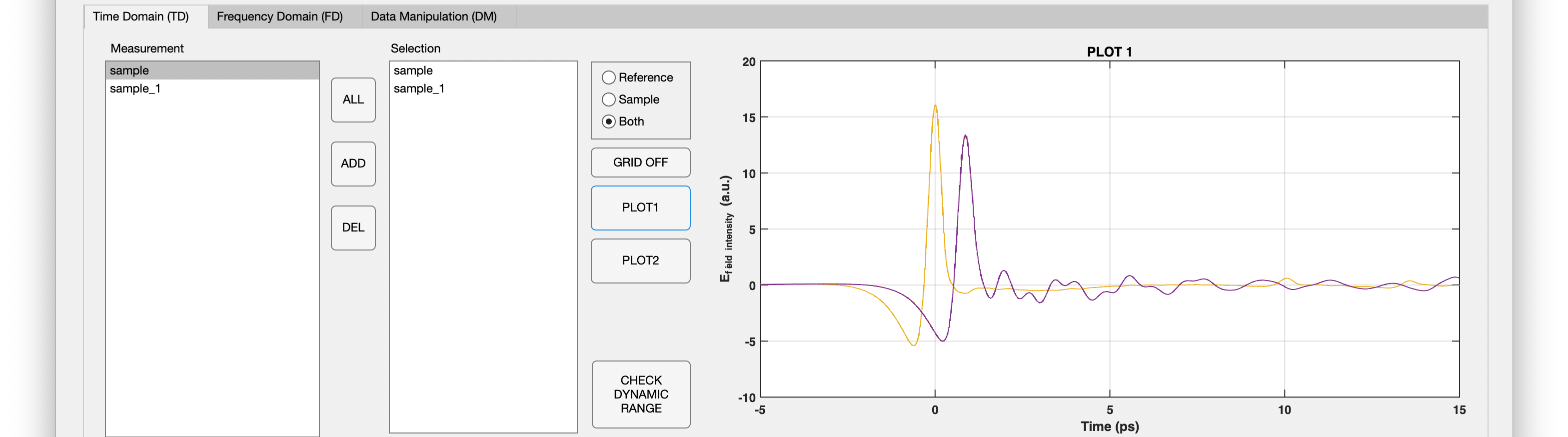
The measurement contains waveforms for both the reference and the sample. The default setting (where the “Both” radio button is chosen) will plot both the reference and the sample waveforms. The user can choose the “Reference” or “Sample” radio button to plot only the reference or the sample waveform respectively. This allows the user the visualise the waveforms recorded and select those of interest for fast Fourier transformation (FFT) into the FD.
Fast Fourier Transformation (FFT)
The “FFT Settings” field is designated for the FFT and the FD analysis (see next section). The values assigned in the “FFT Settings” field serves globally for all items in the “Selection” list box.
The mathematical steps on the Fourier Transform we use in Catsper can be found here.
“Frequency range” sets the range of frequencies for the FFT. The default values are 0.2 THz for the minimum frequency and 2.8 THz for the maximum frequency. The user can change these values in corresponding edit fields.
“FFT Upsampling” has default value of zero filling and power of 2. The user can alter this power value by operating the spinner. Upsampling is the process to pad zeros at the high frequency component end on each side of the signal.
“Window function” can either “AUTO WINDOW” at 1st internal reflections (if this button is pushed in) or the user can specify the minimum time and the maximum time. The default values are -10.00 ps and 20.00 ps respectively.
“Apodization Function” allows the user to select an apodization function used from a drop-down list including “Boxcar”, “Hammering”, “Bartlett”, “Blackman”, “Hann”, “Taylor” and “Triang”. The default value is “Boxcar”. An apodization function helps smoothly reduce the edge signal to zero at the boundaries between which the frequencies are chosen for the FFT.
Once the user completes all settings, clicking the “TRANSFORM” button will enable the App to compute the FFT and the “Spectral Resolution (THz)” label will appear above this button. This then prepares the user for the FD analysis outlined in the next section.
“TRANSFORM” button will evaluate the FFT.
Summary of all button functionalities under the “Time Domain” tab
“ALL”: add all data sets from the “Measurement” list box to the “Selection” list box
“ADD”: add chosen data set from the “Measurement” list box to the “Selection” list box
“DEL”: remove chosen data set from the “Selection” list box
“GRID OFF”: turn off the grid lines on the plots
“PLOT1”: reveal the plot on “PLOT 1” area
“PLOT2”: reveal the plot on “PLOT 2” area
“FIND THICKNESS”
“PLOT THICKNESS”
“PLOT REFRACTIVE INDICES”: plot the refractive indices against their data sets
“TRANSFORM”: evaluate the fast Fourier transform for data sets in the “Selection” list box and transfer the data to “FD List” list box under the “Frequency Domain” tab
“LEGEND”: turn on the legend for the data sets
“JET COLORMAP”: change the colour scheme for the curve to jet colourmap
“LOAD TD DATA”: import saved TD data from .mat file
“SAVE TD DATA”: save all TD data from the “Measurement” or “Selection” list box, depending on the user response
“ASSIGN TD DATA IN WORKSPACE”: assign all TD data from the “Measurement” list box to the workspace
Frequency Domain (FD) Tab
Note: Please carry out the TD analysis before commencing the following steps, otherwise, nothing will be displayed in the “FD List” list box.
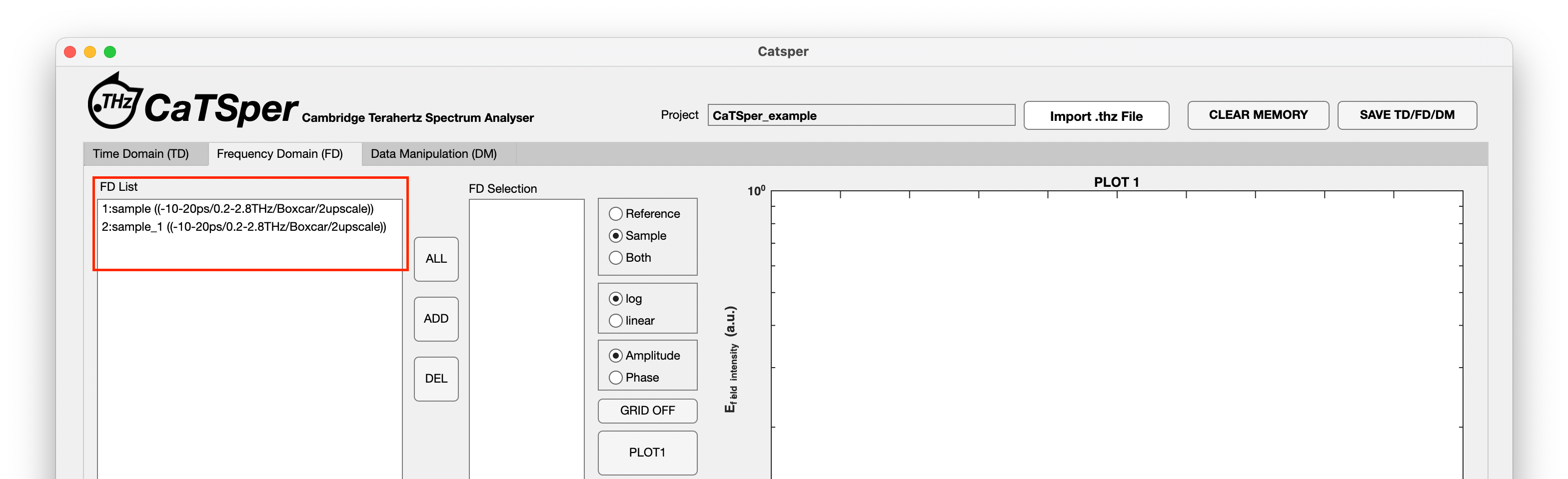
To perform the FD analysis, the user needs to select the “Frequency Domain (FD)” tab at the top left corner of the Catsper user interface to open the FD analysis page.
Data obtained by FFT from TD analysis
Once the FFT is done by clicking the “TRANSFORM” button under the “Time Domain (TD)” tab, the measurement(s) in the “Selection” list box will appear in the “FD list” list box with the following naming structure:
“[Measurement Name] ([Min.Time]-[Max.Time]ps/([Min.Freq.]-[Max.Freq.]THz/[Apodization Function]/[power of upsampling]upscale)”
Choose the FD data for analysis
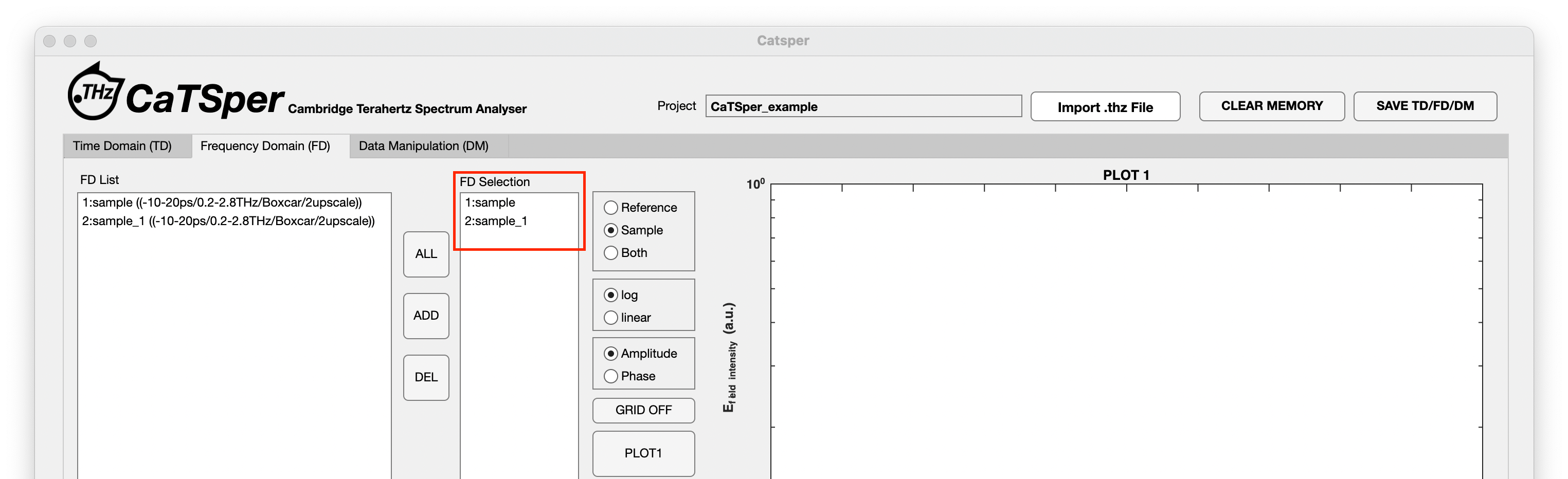
This process is quite the same as the TD analysis. The user can pick those of interest by click the target item (and the selected item will be shaded). The user can click the “ADD” button and measurement name will then appear in the “FD Selection” list box. Please note that only one measurement can be selected each time, so if you want to include all measurements, simply click the “ALL” button and all measurements will be added thereafter. If you want to remove some measurements already in the “FD Selection” list box, choose the target item in the “FD Selection” list box and click the “DEL” button. This item will then disappear from the “FD Selection” list box, however, it can still be found in the “FD List” list box.
Save the list of FD data
Once the FD data have been selected and appeared in the “FD Selection” list box, the user can click the “SAVE FD DATA”. A message box will pop out to ask: “Do you want to save all data?”. If the user return “Yes”, then all list items in the “FD List” list box will be saved in the .mat file, whereas “No, only the selected data” will only save those in the “FD Selection” list box.
Load the list of FD data
Click the “LOAD FD DATA” and choose the .mat file created by the “SAVE FD DATA” functionality. The FD data saved in this file will then be imported to the “FD List” and “FD Selection” list boxes.
Plot the FD data
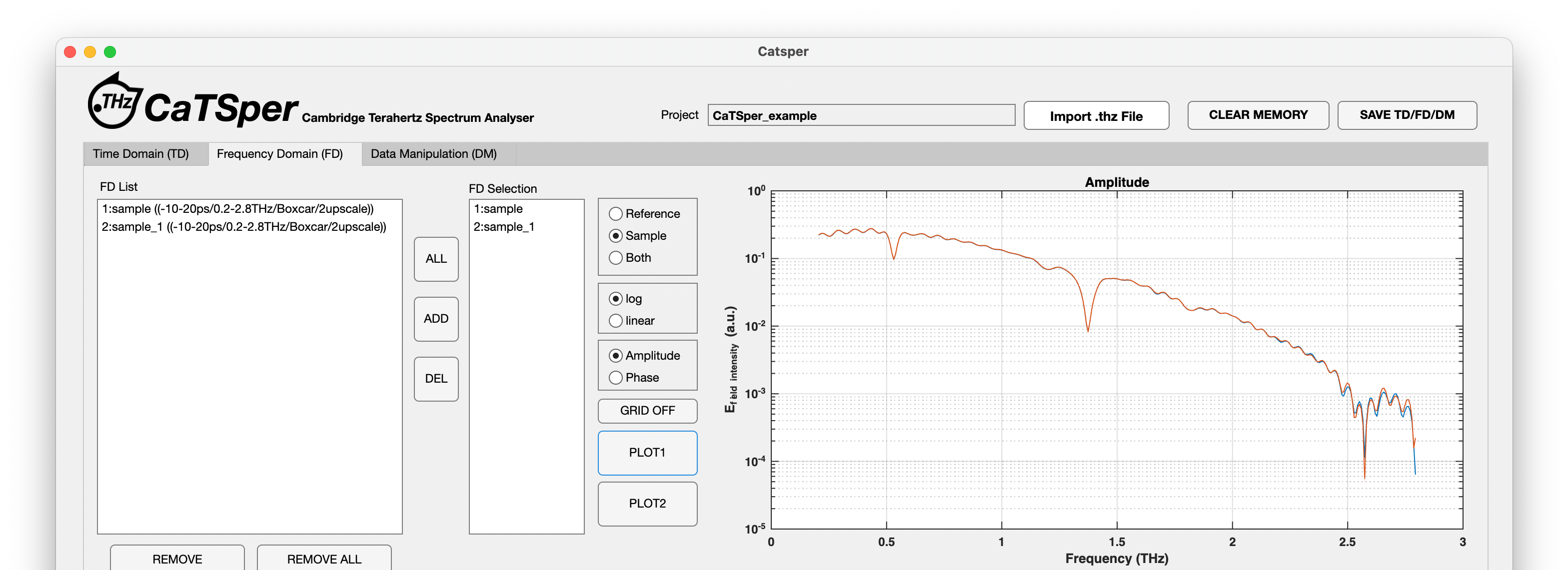
The operations are like those in the “Plot the TD data” section. Similarly, the plot can only be done once the data are selected and displayed in the “Selection” list box. This will enable the user to visualise the FD waveforms before applying any bandwidth filter.
Clicking the “PLOT1” button will generate the waveform plot on the “PLOT 1” axis whilst such plot will appear on the “PLOT 2” axis if the “PLOT2” button is pushed in. The user can plot the same measurement on both axes. These operations will generate the plots for all FD data in the “FD Selection” list box. If the user wishes to remove certain FD data from the plot, click the unwanted data and press “DEL”. Then click either the “PLOT1” or “PLOT2” button, and the new plot will override the previous plot.
The default setting for the plot is plot “Sample” waveforms under the “log” scale with “Amplitude” on the vertical axis. The user can customise the following changes by choosing a different radio button to the right-hand-side of the “FD selection” list box:
“Reference”: plot the reference waveforms only;
“Sample”: plot the sample waveforms only;
“Linear”: use the linear scale;
“Phase”: plot the phase (in degree form) against frequency (THz).
An example of plotting “Both” in the “Log” space:
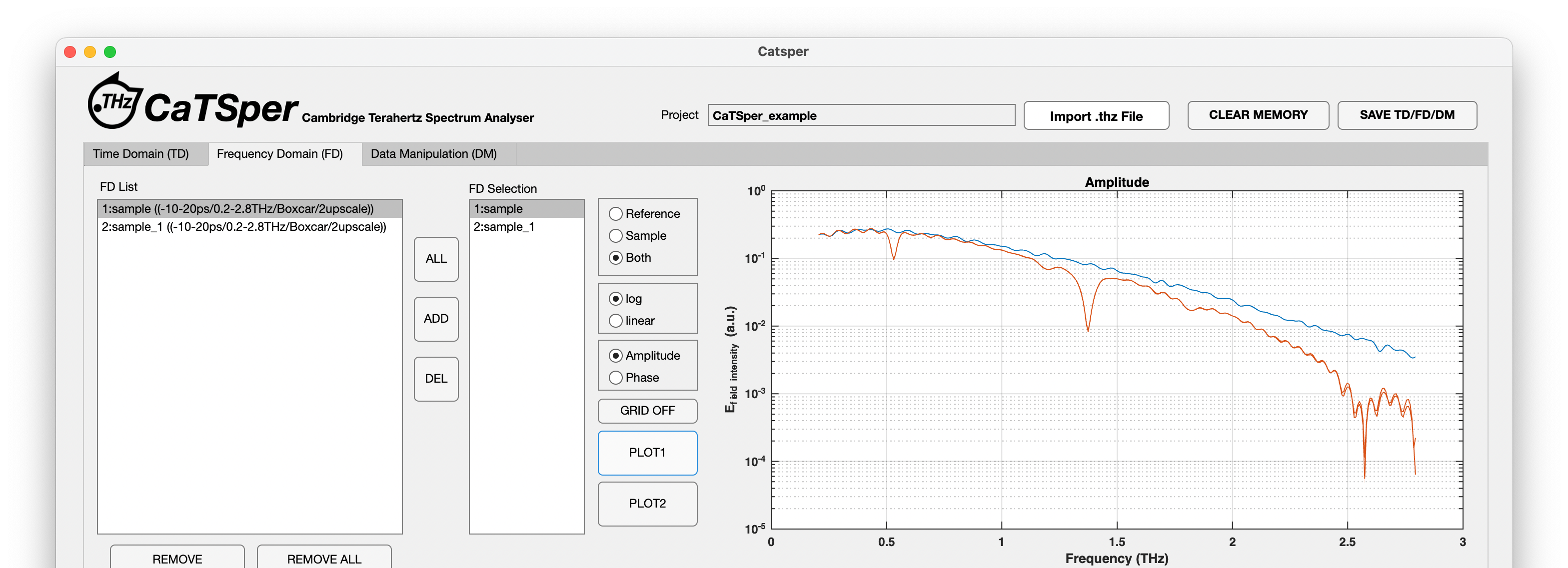
The user needs to click either the “PLOT1” or “PLOT2” button to update the plot or axes.
The default settings will generate the grid on the plot. If the user wants to turn off the grid line, press the “GRID OFF” button (and it will turn grey) and click either the “PLOT1” or “PLOT2” button to update the plot.
FD data analysis
In the “FD Data Analysis” field, the user can apply bandwidth filter to improve the signal quality for, extract and plot the “Transmittance”, “Absorption”, “Refractive Index” and “Dielectric Constant” from the measurements.
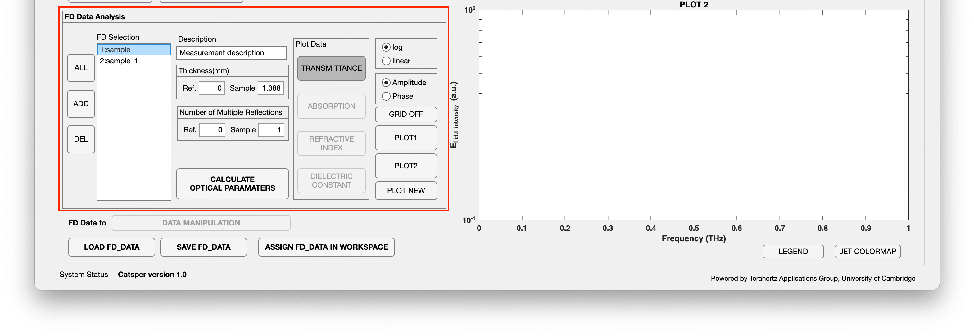
The user needs to select the FD data for analysis from the “FD List” list box and press the “ADD” button in the “FD Data Analysis” field to import them into the “FD Selection” list box in this field. Note that this procedure is done separately to that outlined in the “Plot the FD data section”.
The “ALL” button loads all data from the “FD list” list box to the “FD Selection” list box whilst the “DEL” removes the selected item from the “FD Selection” list box.
The “CALCULATE OPTICAL PARAMETERS” button will then evaluate the absorption, refractive index, and the dielectric constant for each item listed in the “FD Selection”. The mathematical steps Catsper follows can be found here.
The user can choose to plot and preview these constants under the “Frequency Domain (FD)” tab. In the “Plot Data” section, the “Transmittance” button can be pushed in, and its plot can be displayed prior to the absorption, refractive index, and the dielectric constant evaluation using the “CALCULATE” button. However, “Absorption”, “Refractive Index”, and the “Dielectric Constant” buttons are greyed out and can only be pushed in once these constants are evaluated.
The default setting pushes the “Transmittance” button in whereas another button needs to be pushed in when that constant can be plotted. For instance, if the user wished to plot absorption on the vertical axis on the plot area 2, the user needs to push in the “ABSORPTION” button first and click “PLOT 2” to the right-hand-side:
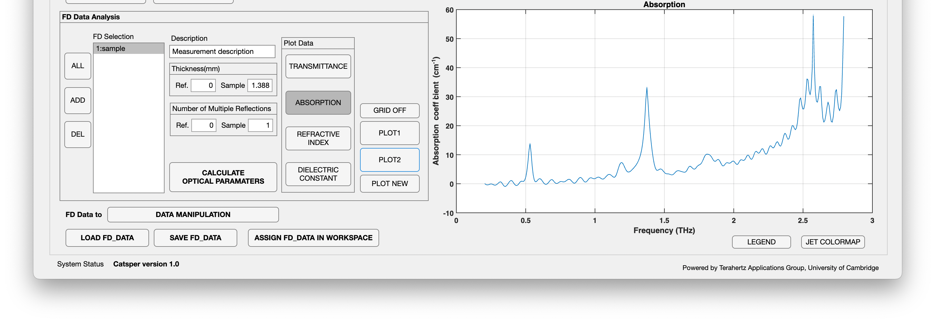
The “PLOT NEW” button to the bottom right corner of the “FD Data Analysis” field will open a new window and display the plot on this figure window.
Once the user is satisfied with the FD data analysis, clicking “DATA MANIPULATION” button will transfer the evaluated transmittance, absorption, refractive index, and the dielectric constant to the “Data Manipulation (DM)” tab. This will also open the “Data Manipulation (DM)” tab for the user.

Summary of all button functionalities under the “Frequency Domain” tab
“ALL”: add all data sets from the “FD List” list box to the “FD Selection” list box
“ADD”: add chosen data set from the “FD List” list box to the “FD Selection” list box
“DEL”: remove chosen data set from the “FD Selection” list box
“GRID OFF”: turn off the grid lines on the plots
“PLOT1”: reveal the plot on “PLOT 1” area
“PLOT2”: reveal the plot on “PLOT 2” area
“PLOT NEW”: reveal the plot on a new figure window
“CALCULATE”: evaluate the “Absorption”, “Refractive Index”, and the “Dielectric Constant” for the data sets in the “FD Selection” list box
“BANDWIDTH FILTER”: open the bandwidth filter window
“LEGEND”: turn on the legend for the data sets
“DATA MANIPULATION”: transfer the data sets with calculated “transmittance”, “Absorption”, “Refractive Index”, and the “Dielectric Constant” to “Available Data Set” box under the “Data Manipulation” tab and open the “Data Manipulation” tab
“JET COLORMAP”: change the colour scheme for the curve to jet colourmap
“LOAD FD DATA”: import saved FD data from .mat file
“SAVE FD DATA”: save all FD data from the “FD List” or “FD Selection” list box, depending on the user response
“ASSIGN FD DATA IN WORKSPACE”: assign all FD data from the “FD List” list box to the workspace
Data Manipulation (DM) Tab
Note: Please carry out the FD analysis before commencing the following steps, otherwise, nothing will be displayed in the “Available Data Set” box.
Define the variables for the plot
The user will find the “STEP 1” field dedicated for this functionality. It allows the user to choose three variables and plot the variables on the “PLOT 1” area. The variable on the x-axis (or horizontal axis) is chosen from a drop-down list whilst the y-axis (or vertical axis) can be assigned to more variables (see later).
The data sets in the “Available Data Set” box are transferred from the “FD Domain” tab. The user will find a series of number separated by space. The numbering corresponds to those listed in the “FD Selection” list box on the “FD Domain” tab. If there is nothing shown in the “Available Data Set” box, please check your FD data analysis and ensure you have transferred the data correctly to this tab.
To import the data set for the plot, the user needs to define the “Source Data Set” box. This can be done by inputting the number(s) of the data set and separate them by space. For example, provided “1 2 3 4 5 6 7 8 9 10” is displayed in the “Available Data Set” box, the user can change the value of the “Source Data Set” box to “1 3 7 10” if only these data sets are required for the plot. Alternatively, if all these ten data sets are required, the user can press the “IMPORT ALL DATA” button to import “1 2 3 4 5 6 7 8 9 10” in one step. A convenient step if only “1 2 3 4 7 8 9 10” is required for the plot can be done by import all data first and remove the unwanted data set “5 6” from the “Source Data Set” box.
“Define variables” allows the user to assign values selected from a drop-down box from the data sets to three variables, A, B and C. These values are
“frequency”: Frequency
“ref_amplitude”: Refence amplitude
“ref_phase”: Reference phase
“sam_amplitude”: Sample amplitude
“sam_phase”: Sample phase
“transmit_amplitude”: Transmittance amplitude
“transmit_phase”: Transmittance phase
“refractiveindex”: Refractive index
“absorption”: Absorption
“extinction”: Extinction coefficient
“ereal”: Real part of extinction coefficient
“eimag”: Imaginary part of extinction coefficient
For example, A, B, and C can be defined as “absorption”, “sam_amplitude”, and “ref_amplitude” respectively. (These example variable definition will be carried forward.)
It follows by assigning the x-axis and y-axis data. The “X-axis Data” is selected from a drop-down box whilst “Y-axis Data Formulation” enables the user to use an equation formulated by A, B, and/or C. To illustrate, if the user wants to plot (sample amplitude) – (reference amplitude) on the y-axis against (frequency) on the x-axis, the user needs to type the formula “B-C” in the “Y-axis Data Formulation” box and pick “frequency” from the drop-down box. To evaluate the value for the y-axis, press “CALCULATE”. When the evaluation finishes, the “Number of Data” box will reveal the number of data sets used for the plot and the “PLOT (individual data sets)” and “PLOT (mean and range)” that previous greyed out will be available.
“PLOT (individual data sets)” will plot each data set as a separate curve; “PLOT (mean and range)” will evaluate the mean of each y-axis value at its corresponding x-axis value and plot the average value curve as well as the region (shaded in red) where all data sets reside.
All these plots will be shown in the “PLOT 1” area.
For instance, if the user plot “absorption” and “frequency” on the y-axis and x-axis respectively, using all available data sets:
Click ““IMPORT ALL DATA””;
Define A for “absorption” (B and C can remain as their default values);
Choose “frequency” for “X-axis Data”;
Type “A” in the “Y-axis Data Formulation” box;
Click “CALCULATE”;
Check if the value of “Number of Data” should be changed to “36”;
Click the “PLOT (individual data sets)” gives the following plot in “PLOT 1”:
Otherwise, click the “PLOT (mean and range)” reveal the following plot “PLOT 1”:
The user has prepared the data set and can proceed to the next step for data extraction outlined in the next section.
Extract data from frequency domain spectra
The bottom half of the “Data Manipulation (DM)” tab is dedicated for Catsper to extract values at chosen frequency or find the peak above certain frequency.
Frequency Base Tab
Under the “Frequency Base” tab, the user can extract values at chosen terahertz frequency specified in the “Get Data from Frequency(THz)” box. The “DISPLAY X LINES” button will add a dashed red line to this specified frequency.
“REARRANGE DATA” button gets the values on the y-axis from “PLOT 1” at the specified frequency and display the “Measurement” name (if pre-defined) and “X-axis data”.
“PLOT” button will plot the “Y-axis data” against “X-axis data” on the area to the right-hand-side. The user can define the “X-Label” (default value “Temperature (K)”) and “Y-Label” by changing the corresponding boxes.
Peak Base Tab
Under the “Peak Base” tab, the user can ask Catsper to find the peak on the frequency domain spectrum and plot the y-axis values where the peak is found against the data set number. The user can find the algorithm Catsper uses to find peaks here.
The user needs to define the minimum peak prominence (default value “0”), lower frequency limit (default value “1 THz”) and the number of peaks (default value “1”). Then, by clicking the “REARRANGE DATA” button, Catsper will locate the peaks above the chosen frequency limit.
“PLOT” button will plot the “Y-axis data” where the peak is found against the individual data set on the area to the right-hand-side. The user can define the “X-Label” (default value “Temperature (K)”) and “Y-Label” by changing the corresponding boxes.
Summary of all button functionalities under the “Data Manipulation” tab
“IMPORT ALL DATA”: add all data sets from the “Available Data Set” box to the “Source Data Set” box
“PLOT (individual data sets)”: plot each data set as a separate curve
“PLOT (mean and range)”: evaluate the mean of each y-axis value at its corresponding x-axis value and plot the average value curve as well as the region (shaded in red) where all data sets reside
“CALCULATE”: arrange the chosen x-axis and y-axis variable to the respective axes
“DISPLAY X LINES”: add a dashed red line to this specified frequency
“REARRANGE DATA” (frequency base): get the values on the y-axis from “PLOT 1” at the specified frequency and display the “Measurement” name (if pre-defined) and “X-axis data”
“REARRANGE DATA” (peak base): locate the peaks above the chosen frequency limit
“PLOT”: reveal the plot for the frequency base or peak base analysis
“PLOT (in a new figure)”: reveal the plot on a new figure window
“SAVE DM DATA”: save all data processed in DM to a .mat file
“ASSIGN FD DATA IN WORKSPACE”: assign all data processed in DM to the workspace as “DM_data”